Time signal classification using Convolutional Neural Network in TensorFlow - Part 2

After transforming 1D time domain data series into frequency 2D maps in part 1 of this miniseries, we’ll now focus on building the actual Convolutional Neural Network binary classification model. The goal is to detect whether the original time domain signal exhibits partial discharge and is likely to result in a power line failure in the future.

Two CNN models of various depth and complexity are presented to discuss the hyperparameters, results and suitability for a given dataset that presents challenges related to limited size and highly unbalanced classes.

Full example repo on GitHub

If you want to get the files for the full example, you can get it from this GitHub repo. You’ll find two files: frequency domain TFRecord transformation.py
CNN_TFR_discharge_detection.py

Dataset Overview

• Individual sample format: 250 x 200 2D tensor
• Train: 8160 samples with an upsampled minority class using custom permutations
• Evaluation: 2178 samples
• Storage: TFRecords with 30 samples per file

TensorFlow Approach

The CNN models are built using the TensorFlow Estimators API, as it provides good flexibility and control over building custom models while allowing more robust data streaming and resource solution. This is highly desirable as we work with fairly large dataset and wish to reduce the costs related to computing resources.

As a result, the input function for the custom estimators will stream the data batch by batch, which allows us to use arbitrary computing resources and the only limitation is the time we are willing to dedicate to training the CNN. To accommodate this solution, the input function uses the TensorFlow Data API and TFRecord iterator. This is extremely convenient solution and the Estimators API will take care of initializing the iterator and setting up the graph.

Input function and Pipeline

The input_fn of the Estimator API serves two purposes:

• Create a dataset to stream parsed data via an iterator
• Establish a pipeline for data transformation before feeding it to the model

The input_fn receives four parameters:

• path to TFRecords
• batch size
• mode (Train = True/False)
• number of epochs

Initiating the dataset

The first step is to initialize the dataset using a data API TFRecordDataset class:

def dataset_input_fn(subfolder, batch_size, train = False, num_epochs=None):
         
    filenames = [file for file in os.listdir(subfolder) if file.endswith('.tfrecord')]
    filenames = [os.path.join(subfolder, file) for file in filenames]
    dataset = tf.data.TFRecordDataset(filenames)

Note that the Estimator API will take care of initializing the iterator, so we do not have to worry about it here as opposed to manually building a graph where you would have to do something like this:

    iterator = dataset.make_initializable_iterator()
    sess.run(iterator.initializer)

Parsing the TFRecords

The second step in the input_fn is to parse the data from TFRecords, where the data is stored as lists with one of the three datatypes (float-, byte- and int64- list):

        features = {
            'signal': tf.FixedLenFeature([50000], dtype=tf.float32),
            'signal_ID': tf.FixedLenFeature([], dtype=tf.int64),
            'measurement_ID': tf.FixedLenFeature([], dtype=tf.int64),
            'label': tf.FixedLenFeature([], dtype=tf.int64)}
        parsed = tf.parse_single_example(record, features)

Pipeline

The parsing and input_fn is an ideal place for building your pipeline. In this example, the pipeline consists of two operations. First, we can assume that any physical effects related to the partial discharge are exhibiting at higher frequencies. This is due to the fact that a partial discharge lasts only a very short time(in the order of microseconds). Therefore, we can easily reduce the feature size by dropping all datapoints representing lower frequencies without losing any valuable information:

        signal_data = tf.reshape(parsed['signal'], [-1, 250, 200])
        #remove low frequency components
        signal_data = tf.slice(signal_data, [0, 2, 0], [1, 240, 200])

We could possibly experiment with removing even more of the low frequency datapoints and reducing the feature tensor dimension.

The second step in the normalization is to scale the data. The following code demonstrates two types of scaling:

• Min/Max with rounding to 0 or 1, creating a black and white feature map
• Scaling to a fixed value, creating a float map where most values lie between 0 and 1, but outliers can reach higher values without reducing most of the information.

        # Perform additional preprocessing on the parsed data.
        bw_data = tf.reshape(tf.sqrt(parsed['signal']), [-1, 250, 200])
        bw_data = tf.slice(bw_data, [0, 2, 0], [1, 240, 200])
        
        # Min max normalization
        bw_data = tf.div(
                tf.subtract(
                    bw_data, 
                    tf.reduce_min(bw_data)
                ), 
                tf.subtract(
                    tf.reduce_max(bw_data), 
                    tf.reduce_min(bw_data)
                )
        )
        bw_data = tf.round(bw_data)
        
        signal_data = tf.reshape(parsed['signal'], [-1, 250, 200])
        #remove low frequency components
        signal_data = tf.slice(signal_data, [0, 2, 0], [1, 240, 200])
        
        #Normalize and scale data
        qube = tf.fill([240,200],1/3)
        signal_data = tf.pow(signal_data,qube)
        signal_data = tf.image.per_image_standardization(signal_data)
        
        norm_max = tf.fill([240,200],6.0)
        signal_data = tf.divide(signal_data,norm_max)

        label = tf.cast(parsed["label"], tf.int32)
    
        return {"signal_data": signal_data, "bw_data": bw_data, "signal_ID": parsed["signal_ID"]}, label

Tip: Manually extracting information from TFRecords

You can easily extract specific parameters from TFRecords without running the Estimator API. Here is an example code snippet that extracts labels from the evaluation set: #%% Get labels from TFR files

with tf.Session() as sess:
    dataset = dataset_input_fn(eval_folder, train = False, batch_size = 2178, num_epochs=1)
    iterator = dataset.make_initializable_iterator()
    sess.run(iterator.initializer)
    batch = iterator.get_next()
    labels = batch[1].eval()

CNN Model #1

The first model consists of four convolutional layers and two dense layers with relu activation functions. Most layers have dropout rates to reduce overfitting as we have a limited training dataset and the training will have to be conducted using multiple epochs. The following visualizations shows the overall CNN architecture:

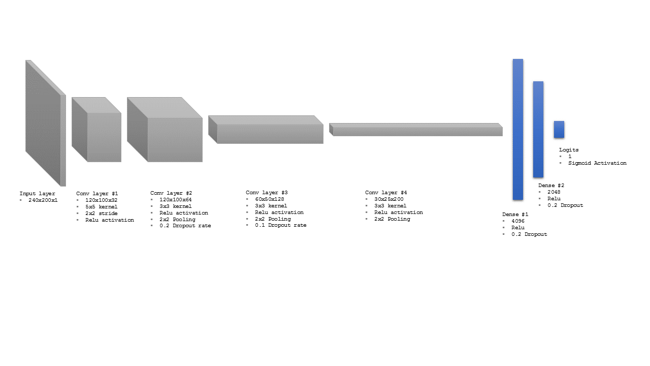
and here is the equivalent python code for TensorFlow Estimators:

#%% Building the CNN Classifier
def cnn_model_fn(features, labels, mode):
  """Model function for CNN."""
  if mode == tf.estimator.ModeKeys.PREDICT:
      pass
  else:    
      labels=tf.reshape(labels,[-1,1])
  input_layer = tf.reshape(features["signal_data"], [-1, 240, 200,1])
  print(input_layer)
  
  # Convolutional Layer #1
  conv1 = tf.layers.conv2d(
      inputs=input_layer,
      filters=32,
      kernel_size=[5, 5],
      strides=(2, 2),
      padding="same",
      activation=tf.nn.relu)
      #Output -1,120,100,32
  print(conv1)

  # Convolutional Layer #2 and Pooling Layer #2
  conv2 = tf.layers.conv2d(
      inputs=conv1,
      filters=64,
      kernel_size=[3, 3],
      padding="same",
      activation=tf.nn.relu)
  #Output -1,120,100,64
  pool2 = tf.layers.max_pooling2d(inputs=conv2, pool_size=[2, 2], strides=2)
  #Output -1,60,50,64
  dropout = tf.layers.dropout(
      inputs=pool2, rate=0.1, training=mode == tf.estimator.ModeKeys.TRAIN)
  
  # Convolutional Layer #3 and Pooling Layer #3
  conv3 = tf.layers.conv2d(
      inputs=dropout,
      filters=128,
      kernel_size=[3, 3],
      padding="same",
      activation=tf.nn.relu)
  #Output -1,60,50,128
  pool3 = tf.layers.max_pooling2d(inputs=conv3, pool_size=[2, 2], strides=2)
  #Output -1,30,25,128
  dropout2 = tf.layers.dropout(
      inputs=pool3, rate=0.1, training=mode == tf.estimator.ModeKeys.TRAIN)
  
  # Convolutional and pooling Layer #4
  conv4 = tf.layers.conv2d(
      inputs=dropout2,
      filters=200,
      kernel_size=[3, 3],
      padding="same",
      activation=tf.nn.relu)
  #Output -1,30,25,200 
  pool4 = tf.layers.max_pooling2d(inputs=conv4, pool_size=[2, 2], strides=2)
  #Output -1,15,12,200

  # Dense Layer
  pool4_flat = tf.reshape(pool4, [-1, 15 * 12 * 200])
  dense = tf.layers.dense(inputs=pool4_flat, units=4096, activation=tf.nn.relu) 
  
  dropout3 = tf.layers.dropout(
      inputs=dense, rate=0.2, training=mode == tf.estimator.ModeKeys.TRAIN)
  
  dense2 = tf.layers.dense(inputs=dropout3, units=2048, activation=tf.nn.relu)
  
  dropout4 = tf.layers.dropout(
      inputs=dense2, rate=0.2, training=mode == tf.estimator.ModeKeys.TRAIN)

  # Logits Layer
  logits = tf.layers.dense(inputs=dropout4, units=1)

Since this is a binary classification problem, we use a sigmoid function to get the prediction probabilities from logits and use a simple rounding function to assign classes based on the calculated probabilities. Similarly, we use a sigmoid cross entropy loss function to navigate the gradients during training optimization:

  predictions = {
      # Generate predictions (for PREDICT and EVAL mode)
      "classes": tf.round(tf.nn.sigmoid(logits)),
      "probabilities": tf.nn.sigmoid(logits, name="probs_tensor"),
      "signal_id": tf.reshape(features["signal_ID"],[-1,1])
  }
  

  if mode == tf.estimator.ModeKeys.PREDICT:
    return tf.estimator.EstimatorSpec(mode, predictions=predictions)

  loss = tf.losses.sigmoid_cross_entropy(multi_class_labels=labels, logits=logits)


  # Configure the Training Op (for TRAIN mode)
  if mode == tf.estimator.ModeKeys.TRAIN:
    
    # Calculate Loss (for both TRAIN and EVAL modes) via cross entropy
    
    optimizer = tf.train.GradientDescentOptimizer(learning_rate=0.001)
    train_op = optimizer.minimize(
        loss=loss,
        global_step=tf.train.get_global_step())
    return tf.estimator.EstimatorSpec(mode=mode, loss=loss, train_op=train_op)

  # Add evaluation metrics (for EVAL mode)
  eval_metric_ops = {
          "accuracy": tf.metrics.auc(
          labels=labels, predictions=predictions["classes"])
    
  }
  return tf.estimator.EstimatorSpec(
      mode=mode, loss=loss, eval_metric_ops=eval_metric_ops)

Training and Evaluation

Since we are dealing with highly imbalanced classes, the standard accuracy metrics for evaluation would be very unreliable. Therefore, custom evaluation using a confusion matrix and Mathews Correlation Coefficient (MCC) is calculated based on the predicted probabilities.

Mathews Correlation matrix:

To do this, we first load the predicted probabilities for the evaluation set and assign classes based on an input threshold value determining the range for class = 1:

def score_model_measurement(probs,threshold):
    predicted = np.array([1 if x > threshold else 0 for x in probs[:,0]])           
    return predicted

Once classes are assigned, the corresponding confusion matrix and MCC is calculated:

#Print confusion matric and calculate Matthews correlation coefficient (MCC) 
def print_metrics(labels, scores):
    conf = confusion_matrix(labels, scores)
    print('                 Confusion matrix')
    print('                 Score positive    Score negative')
    print('Actual positive    %6d' % conf[1,1] + '             %5d' % conf[1,0])
    print('Actual negative    %6d' % conf[0,1] + '             %5d' % conf[0,0])
    print('')
    print('Accuracy  %0.2f' % accuracy_score(labels, scores))
    
    TP = conf[1,1]
    TN = conf[0,0]
    FP = conf[0,1]
    FN = conf[1,0]
    MCC = ((TP*TN) - (FP*FN)) / np.sqrt((TP+FP)*(TP+FN)*(TN+FP)*(TN+FN))
    print('MCC = %0.2f' %MCC)
    return MCC

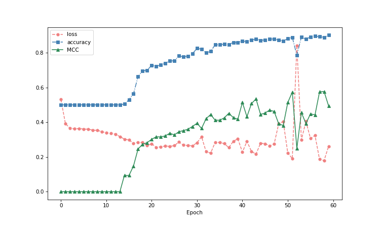
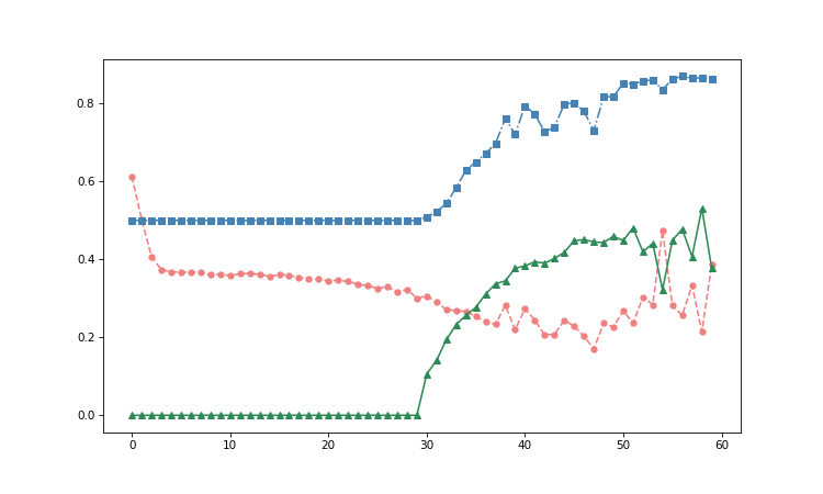
The evaluation routine runs every single epoch and plots the following as a function of the epoch number:

• Training set loss (Sigmoid cross entropy)
• Evaluation set accuracy determined by Area Under Curve (AUC)
• Evaluation set MCC

Following the development of these parameters during the training allows us to determine the predictive power for the minority class, when further learning does not provide further improvement and when we start risking overfitting.

Hyper-parameters:

• Epochs: 60
• Training rate: 0.001
• Batch size: 40
• Shuffle: Yes

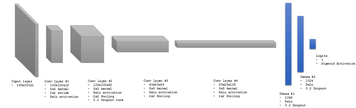
CNN Model #2

Model Architecture

Performance Evaluation Hyper-parameters:

• Epochs: 35
• Training rate: 0.001
• Batch size: 60
• Shuffle: Yes

Conclusion

Both architectures, which mostly differed in the number of features and nodes, showed similar prediction power achieving an accuracy(AUC) of ~0.94 and Mathews Correlation Coefficient around 0.57. For comparison, this is very similar to what we were able to achieve with gradient boosted trees on data from statistical analysis of the time signal. Nevertheless, the construction of the CNN solution was considerably less effort intensive as the CNN automatically extracts the features at a cost of longer training time. If we consider that human capital is more expensive than computing power, this metrics still comes in favour of the CNN.That being said, the ultimate goal is to use an ensemble of classifiers that will take a vote on the final class and further increase the predictive power.

The main difference between the two architectures was in the training time where the model #1 required 255 seconds per 100 steps and model #2 required 150 seconds. Therefore, all other metrics being the same, model #2 would be more favorable as it is faster and requires less computing resources.

Looking at the evaluation plots vs training epoch, we can also estimate that there is very little to no improvement in running the training beyond epoch #40 and we only increase the risk of overfitting.

Example results:

Confusion matrix

                 Score positive    Score negative
Actual positive        90                18
Actual negative       118              1952

Accuracy  0.94
MCC = 0.57

INFO:tensorflow:loss = 0.08221432, step = 10556 (150.680 sec)
INFO:tensorflow:global_step/sec: 0.241183